SPSS Articles
Annotated Output | Factorial ANOVA
Computer Output
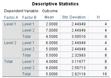
The table of descriptive statistics can be used to determine the inferential statistics.
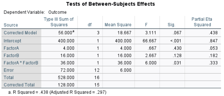
The table of inferential statistics shows the key elements to be calculated.
Calculations
Descriptive Statistics: The descriptive statistics are calculated separately for each group or condition.
Error (Within Groups) Statistics: Within-groups error statistics are a function of the within group variabilities.
\[SS_1 = ( SD_1^2 ) ( df_1 ) = ( 2.44949^2 ) ( 3 ) = 18.000\] \[SS_2 = ( SD_2^2 ) ( df_2 ) = ( 2.44949^2 ) ( 3 ) = 18.000\] \[SS_3 = ( SD_3^2 ) ( df_3 ) = ( 2.44949^2 ) ( 3 ) = 18.000\] \[SS_4 = ( SD_4^2 ) ( df_4 ) = ( 2.44949^2 ) ( 3 ) = 18.000\] \[SS_{ERROR} = SS_1 + SS_2 + SS_3 + SS_4 = 18.000 + 18.000 + 18.000 + 18.000 = 72.000\] \[df_{ERROR} = df_1 + df_2 + df_3 +df_4 = 3 + 3 + 3 + 3 = 12\] \[MS_{ERROR} = \frac{SS_{ERROR}}{df_{ERROR}} = \frac{72.000}{12} = 6.000\]
Grand (or Total) Mean: A grand mean can be determined by taking the weighted average of all of the group means.
\[M_{TOTAL} = \frac{\sum n_{GROUP} (M_{GROUP})}{N} = \frac{ 4 (2.000) + 4 (7.000) + 4 (6.000) + 4 (5.000) }{( 4 + 4 + 4 + 4 )} = 5.000\]
Marginal Means: A level (marginal) mean can be determined by taking the weighted average of the appropriate group means.
For Factor A:
\[M_{A1} = \frac{\sum n_{GROUP} (M_{GROUP})}{N_{LEVEL}} = \frac{ 4 (2.000) + 4 (7.000) }{( 4 + 4 )} = 4.500\] \[M_{A2} = \frac{\sum n_{GROUP} (M_{GROUP})}{N_{LEVEL}} = \frac{ 4 (6.000) + 4 (5.000) }{( 4 + 4 )} = 5.500\]
For Factor B:
\[M_{B1} = \frac{\sum n_{GROUP} (M_{GROUP})}{N_{LEVEL}} = \frac{ 4 (2.000) + 4 (6.000) }{( 4 + 4 )} = 4.000\] \[M_{B2} = \frac{\sum n_{GROUP} (M_{GROUP})}{N_{LEVEL}} = \frac{ 4 (7.000) + 4 (5.000) }{( 4 + 4 )} = 4.000\]
Effect (Between Groups) Statistics: The Model statistics represent the overall differences among the groups. The Factor A and Factor B statistics are a function of the level (marginal) means and sample sizes. The interaction statistics reflect the between-groups variability not accounted for by the factors individually.
For the Model:
\[SS_{MODEL} = \sum n_{GROUP} (M_{GROUP} - M_{TOTAL})^2 = 4 ( 2.000 - 5.000 )^2 + 4 ( 7.000 - 5.000 )^2 + 4 ( 6.000 - 5.000 )^2 + 4 ( 5.000 - 5.000 )^2 = 56.000\] \[df_{MODEL} = \text{# groups} − 1 = 4 − 1 = 3\]
For Factor A:
\[SS_{FACTORA} = \sum n_{LEVEL} (M_{LEVEL} - M_{TOTAL})^2 = 8 ( 4.500 - 5.000 )^2 + 8 ( 5.500 - 5.000 )^2 = 4.000\] \[df_{FACTORA} = \text{# levels} − 1 = 2 − 1 = 1\] \[MS_{FACTORA} = \frac{SS_{FACTORA}}{df_{FACTORA}} = \frac{4.000}{1} = 4.000\]
For Factor B:
\[SS_{FACTORB} = \sum n_{LEVEL} (M_{LEVEL} - M_{TOTAL})^2 = 8 ( 4.000 - 5.000 )^2 + 8 ( 6.000 - 5.000 )^2 = 16.000\] \[df_{FACTORB} = \text{# levels} − 1 = 2 − 1 = 1\] \[MS_{FACTORB} = \frac{SS_{FACTORB}}{df_{FACTORB}} = \frac{16.000}{1} = 16.000\]
For the Interaction:
\[SS_{INTER} = SS_{MODEL} - SS_{FACTORA} - SS_{FACTORB} = 56.000 - 4.000 - 16.000 = 36.000\] \[df_{INTER} = df_{MODEL} - df_{FACTORA} - df_{FACTORB} = 3 - 1 - 1 = 1\] \[MS_{INTER} = \frac{SS_{INTER}}{df_{INTER}} = \frac{36.000}{1} = 36.000\]
Statistical Significance: The F statistic is the ratio of the between-and within-group variance estimates.
For the Factor A Main Effect:
\[F = \frac{MS_{FACTORA}}{MS_{ERROR}} = \frac{4.000}{6.000} = 0.667\]With dfFACTORA = 1 and dfERROR = 12, FCRITICAL = 4.747
Because FFACTORA < FCRITICAL, p > .05
This would not be considered a statistically significant finding.
For the Factor B Main Effect:
\[F = \frac{MS_{FACTORB}}{MS_{ERROR}} = \frac{16.000}{6.000} = 2.667\]With dfFACTORB = 1 and dfERROR = 12, FCRITICAL = 4.747
Because FFACTORB < FCRITICAL, p > .05
This would not be considered a statistically significant finding.
For the Interaction:
\[F = \frac{MS_{INTER}}{MS_{ERROR}} = \frac{36.000}{6.000} = 6.000\]With dfINTER = 1 and dfERROR = 12, FCRITICAL = 4.747
Because FINTER > FCRITICAL, p < .05
This would be considered a statistically significant finding.
Effect Size: The partial eta-squared statistic is a ratio of the between-subjects effect and the remaining variability (Sum of Squares) estimates after within-subjects error has been partialled out.
For the Factor A Main Effect:
\[\text{Partial} \; \eta^2 = \frac{SS_{FACTORA}}{( SS_{FACTORA} + SS_{ERROR} )} = \frac{4.000}{( 4.000 + 72.000 )} = 0.053\]Thus, 5.3% of the variability among the scores is accounted for by Factor A.
For the Factor B Main Effect:
\[\text{Partial} \; \eta^2 = \frac{SS_{FACTORB}}{( SS_{FACTORB} + SS_{ERROR} )} = \frac{16.000}{( 16.000 + 72.000 )} = 0.182\]Thus, 18.2% of the variability among the scores is accounted for by Factor B.
For the Interaction:
\[\text{Partial} \; \eta^2 = \frac{SS_{INTER}}{( SS_{INTER} + SS_{ERROR} )} = \frac{36.000}{( 36.000 + 72.000 )} = 0.333\]Thus, 33.3% of the variability among the scores is accounted for by interaction of Factor A and Factor B.
Confidence Intervals: For Factorial ANOVA, calculate the confidence intervals around (centered on) each mean separately (not shown here).
APA Style
The Factorial ANOVA provides statistics for the main effects and interactions in a factorial design. Each effect would be summarized in a style analogous to a One Way ANOVA.
A 2 (Factor A) x 2 (Factor B) ANOVA indicated a small and non-statistically significant main effect for Factor A, F(1,12) = 0.67, p = .430, partial η2 = .05, and for Factor B, F(1,12) = 2.67, p = .128, partial η2 = .18. In contrast, the interaction was large in magnitude and statistically significant, F(1,12) = 6.00, p = .031, partial η2 = .33.
Typically, the means, standard deviations, and confidence intervals would be presented in a table or figure associated with this text.