jamovi Articles
Annotated Output | Mixed ANOVA
Computer Output
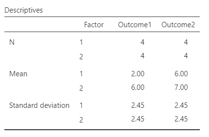
The table of descriptive statistics can be used to determine the inferential statistics.
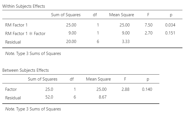
The table of inferential statistics shows the key elements to be calculated.
Calculations
Descriptive Statistics: The descriptive statistics are calculated separately for each group or condition.
Grand (or Total) Mean: A grand mean can be determined by taking the weighted average of all of the group means.
\[M_{TOTAL} = \frac{\sum n_{GROUP} (M_{GROUP})}{N} = \frac{ 4 (2.000) + 4 (6.000) + 4 (6.000) + 4 (7.000) }{( 4 + 4 + 4 + 4 )} = 5.250\]
Subject Means: Each subject in the study would have an average score across the time points.
\[M_{S1} = \frac{0.000 + 4.000}{2} = 2.000\] \[M_{S2} = \frac{0.000 + 7.000}{2} = 3.500\] \[M_{S3} = \frac{3.000 + 4.000}{2} = 3.500\] \[M_{S4} = \frac{5.000 + 9.000}{2} = 7.000\] \[M_{S5} = \frac{4.000 + 9.000}{2} = 6.500\] \[M_{S6} = \frac{7.000 + 6.000}{2} = 6.500\] \[M_{S7} = \frac{4.000 + 4.000}{2} = 4.000\] \[M_{S8} = \frac{9.000 + 9.000}{2} = 9.000\]
Marginal Means: A level (marginal) mean can be determined by taking the weighted average of the appropriate group means.
For Factor:
\[M_{FACTOR1} = \frac{\sum n_{GROUP} (M_{GROUP})}{N_{LEVEL}} = \frac{ 4 (2.000) + 4 (6.000) }{( 4 + 4 )} = 4.000\] \[M_{FACTOR2} = \frac{\sum n_{GROUP} (M_{GROUP})}{N_{LEVEL}} = \frac{ 4 (6.000) + 4 (7.000) }{( 4 + 4 )} = 6.500\]
For Time:
\[M_{TIME1} = \frac{\sum n_{GROUP} (M_{GROUP})}{N_{LEVEL}} = \frac{ 4 (2.000) + 4 (6.000) }{( 4 + 4 )} = 4.000\] \[M_{TIME2} = \frac{\sum n_{GROUP} (M_{GROUP})}{N_{LEVEL}} = \frac{ 4 (6.000) + 4 (7.000) }{( 4 + 4 )} = 6.500\]
Between-Subjects Error Statistics: Between-subjects error refers to average differences across the participants within each Factor level.
\[SS_{ERROR(BETWEEN)} = \sum (\text{number of Time points}) (M_{SUBJECT} - M_{FACTOR\;LEVEL})^2 = \left[2(2.000-4.000)^2 + 2(3.500-4.000)^2 + 2(3.500-4.000)^2 + 2(7.000-4.000)^2\right] + \left[2(6.500-6.500)^2 + 2(6.500-6.500)^2 + 2(4.000-6.500)^2 + 2(9.000-6.500)^2\right] = 52.000\] \[df_{ERROR(BETWEEN)} = (\text{# levels of Factor})(\text{# subjects per level} - 1) = (2)(4-1) = 6\] \[MS_{ERROR(BETWEEN)} = \frac{SS_{ERROR(BETWEEN)}}{df_{ERROR(BETWEEN)}} = \frac{52.000}{6} = 8.667\]
Within-Subjects Variability: The within-subjects variability reflects person-by-time variability.
\[SS_{SUBJECTS} = \sum (Y - M_{SUBJECT})^2 = (0-2)^2 + (4-2)^2 + (0-3.5)^2 + (7-3.5)^2 + (3-3.5)^2 + (4-3.5)^2 + (5-7)^2 + (9-7)^2 + (4-6.5)^2 + (9-6.5)^2 + (7-6.5)^2 + (6-6.5)^2 + (4-4)^2 + (4-4)^2 + (9-9)^2 + (9-9)^2 = 54.000\] \[df_{SUBJECTS} = (\text{number of subjects})(\text{# time points} - 1) = (8)(2-1) = 8\]
Between-Subjects Effect Statistics: The between-subjects effect (Factor) is a function of the marginal means and sample sizes.
\[SS_{FACTOR} = \sum n_{LEVEL} (M_{LEVEL} - M_{TOTAL})^2 = 8(4.000 - 5.250)^2 + 8(6.500 - 5.250)^2 = 25.000\] \[df_{FACTOR} = \text{# levels of Factor} - 1 = 2 - 1 = 1\] \[MS_{FACTOR} = \frac{SS_{FACTOR}}{df_{FACTOR}} = \frac{25.000}{1} = 25.000\]
Within-Subjects Effect Statistics: The within-subjects effects include the main effect of Time and the Factor × Time interaction.
For Time:
\[SS_{TIME} = \sum n_{LEVEL} (M_{LEVEL} - M_{TOTAL})^2 = 8(4.000 - 5.250)^2 + 8(6.500 - 5.250)^2 = 25.000\] \[df_{TIME} = \text{# levels of Time} - 1 = 2 - 1 = 1\] \[MS_{TIME} = \frac{SS_{TIME}}{df_{TIME}} = \frac{25.000}{1} = 25.000\]
For the Interaction:
\[SS_{INTERACTION} = \sum n_{GROUP} (M_{GROUP} - M_{FACTOR} - M_{TIME} + M_{TOTAL})^2 = 4(2.000 - 4.000 - 4.000 + 5.250)^2 + 4(6.000 - 4.000 - 4.000 + 5.250)^2 + 4(6.000 - 6.500 - 4.000 + 5.250)^2 + 4(7.000 - 6.500 - 6.500 + 5.250)^2 = 9.000\] \[df_{INTERACTION} = (\text{# levels of Factor} - 1)(\text{# levels of Time} - 1) = (2 - 1)(2 - 1) = 1\] \[MS_{INTERACTION} = \frac{SS_{INTERACTION}}{df_{INTERACTION}} = \frac{9.000}{1} = 9.000\]
Within-Subjects Error Statistics: After removing the Time effect and the Interaction effect from the total within-subjects variability, the remaining variation is the within-subjects error term.
\[SS_{ERROR(WITHIN)} = SS_{SUBJECTS} - SS_{TIME} - SS_{INTERACTION} = 54.000 - 25.000 - 9.000 = 20.000\] \[df_{ERROR(WITHIN)} = df_{SUBJECTS} - df_{TIME} - df_{INTERACTION} = 8 - 1 - 1 = 6\] \[MS_{ERROR(WITHIN)} = \frac{SS_{ERROR(WITHIN)}}{df_{ERROR(WITHIN)}} = \frac{20.000}{6} = 3.333\]
Statistical Significance: Each F statistic is the ratio of an effect mean square to its corresponding error mean square in the correct stratum.
For the Factor Main Effect:
\[F_{FACTOR} = \frac{MS_{FACTOR}}{MS_{ERROR(BETWEEN)}} = \frac{25.000}{8.667} = 2.885\]With dfFACTOR = 1 and dfERROR(BETWEEN) = 6, p = .140
This would not be considered a statistically significant finding.
For the Time Main Effect:
\[F_{TIME} = \frac{MS_{TIME}}{MS_{ERROR(WITHIN)}} = \frac{25.000}{3.333} = 7.500\]With dfTIME = 1 and dfERROR(WITHIN) = 6, p = .034
This would be considered a statistically significant finding.
For the Interaction:
\[F_{INTERACTION} = \frac{MS_{INTERACTION}}{MS_{ERROR(WITHIN)}} = \frac{9.000}{3.333} = 2.700\]With dfINTERACTION = 1 and dfERROR(WITHIN) = 6, p = .152
This would not be considered a statistically significant finding.
Effect Size: The partial eta-squared statistic is a ratio of each effect Sum of Squares and the remaining variability after that effect’s corresponding error term has been partialled out.
For the Factor Main Effect:
\[\text{Partial} \; \eta^2 = \frac{SS_{FACTOR}}{( SS_{FACTOR} + SS_{ERROR(BETWEEN)} )} = \frac{25.000}{( 25.000 + 52.000 )} = 0.325\]Thus, 32.5% of the variability among the scores is accounted for by Factor.
For the Time Main Effect:
\[\text{Partial} \; \eta^2 = \frac{SS_{TIME}}{( SS_{TIME} + SS_{ERROR(WITHIN)} )} = \frac{25.000}{( 25.000 + 20.000 )} = 0.556\]Thus, 55.6% of the variability among the scores is accounted for by Time.
For the Interaction:
\[\text{Partial} \; \eta^2 = \frac{SS_{INTERACTION}}{( SS_{INTERACTION} + SS_{ERROR(WITHIN)} )} = \frac{9.000}{( 9.000 + 20.000 )} = 0.310\]Thus, 31.0% of the variability among the scores is accounted for by the Factor × Time interaction.
Confidence Intervals: For Mixed ANOVA, calculate the confidence intervals around (centered on) each mean separately (not shown here).
APA Style
The mixed ANOVA provides statistics for the main effects and interaction in a mixed design. Each effect is summarized below in APA style, using the actual R output values:
A 2 (Factor) × 2 (Time) mixed ANOVA showed that the small main effect of Factor was not statistically significant, F(1,6) = 2.89, p = .140, partial η2 = .33, nor was the moderately sized interaction, F(1,6) = 2.70, p = .152, partial η2 = .31. However, the large main effect of Time was statistically significant, F(1,6) = 7.50, p = .034, partial η2 = .56.
Typically, the means, standard deviations, and confidence intervals would be presented in a table or figure associated with this text.