SPSS Articles
Annotated Output | One Sample t Test
Computer Output
The table of descriptive statistics can be used to determine the inferential statistics.

The table of inferential statistics shows the key elements to be calculated.
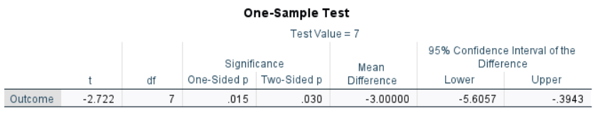
Calculations
Descriptive Statistics: The values of the one-sample statistics are identical to the values that would be provided by the “Descriptives” procedure.
Standard Error of the Mean: The standard error of the mean provides an estimate of how spread out the distribution of all possible random sample means would be.
\[SE_M = \frac{SD}{\sqrt{N}} = \frac{3.117}{\sqrt{8}} = 1.102\]
Mean Difference (Raw Effect): The Mean Difference is the difference between the sample mean and a user-specified test value or population mean.
\[M_{DIFF} = M - \mu = 4.000 − 7.000 = −3.000\]
Statistical Significance: The t statistic is the ratio of the mean difference (raw effect) to the standard error of the mean.
\[t = \frac{M_{DIFF}}{SE_M} = \frac{-3.000}{1.102} = -2.722\]With df = 7, tCRITICAL = 2.365
Because t > tCRITICAL, p < .05
This would be considered a statistically significant finding.
Confidence Interval: For this design, the appropriate confidence interval is around (centered on) the mean difference (raw effect).
\[CI_{DIFF} = M_{DIFF} \pm (t_{CRITICAL} ) (SE_M) = -3.000 \pm (2.365) (1.102) = [ -5.606, -0.394 ]\]Thus, the researcher concludes that the true population mean difference is somewhere between -5.606 and -0.394 (knowing that the estimate could be wrong).
Effect Size: Cohen’s d Statistic provides a standardized effect size for the mean difference (raw effect).
\[d = \frac{M_{DIFF}}{SD} = \frac{-3.000}{3.117} = 0.963\]Given Cohen’s heuristics for interpreting effect sizes, this would be considered a large effect.
APA Style
For this analysis, a sample mean has been compared to a user-specified test value (or a population mean). Thus, the summary and the inferential statistics focus on that difference.
A one sample t test showed that the difference in Outcome scores between the current sample (N = 8, M = 4.00, SD = 3.12) and the hypothesized value (7.00) was large and statistically significant, t(7) = -2.72, p = .030, 95% CI [-5.61, -.39], d = -0.96.