This page examines a two-factor mixed design (one between-subjects and one within-subjects factor) using raw data input, focusing on omnibus and simple effects analyses.
Preliminary Tasks
Data Entry
This code inputs the variable names and creates a viewable data frame.
Factor <- c(rep(1, 10), rep(2, 10))
Factor <- factor(Factor, levels = c(1, 2), labels = c("Level1", "Level2"))
Outcome1 <- c(6, 8, 6, 8, 10, 8, 10, 9, 8, 7, 5, 9, 10, 9, 11, 4, 11, 7, 6, 8)
Outcome2 <- c(7, 13, 11, 10, 13, 8, 11, 14, 12, 11, 7, 8, 7, 11, 10, 7, 8, 4, 8, 10)
Outcome3 <- c(9, 16, 11, 12, 15, 13, 9, 14, 11, 10, 8, 6, 8, 11, 5, 7, 9, 3, 6, 7)
MixedData <- construct(Factor, Outcome1, Outcome2, Outcome3)
Summary Statistics
This code provides a table of summary statistics and a table of correlations and then retain them for the subsequent analyses.
(MixedData) |> focus(Outcome1, Outcome2, Outcome3) |> describeMoments(by = Factor) |> retain(MixedMoments)
(MixedData) |> focus(Outcome1, Outcome2, Outcome3) |> describeCorrelations(by = Factor) |> retain(MixedCorr)
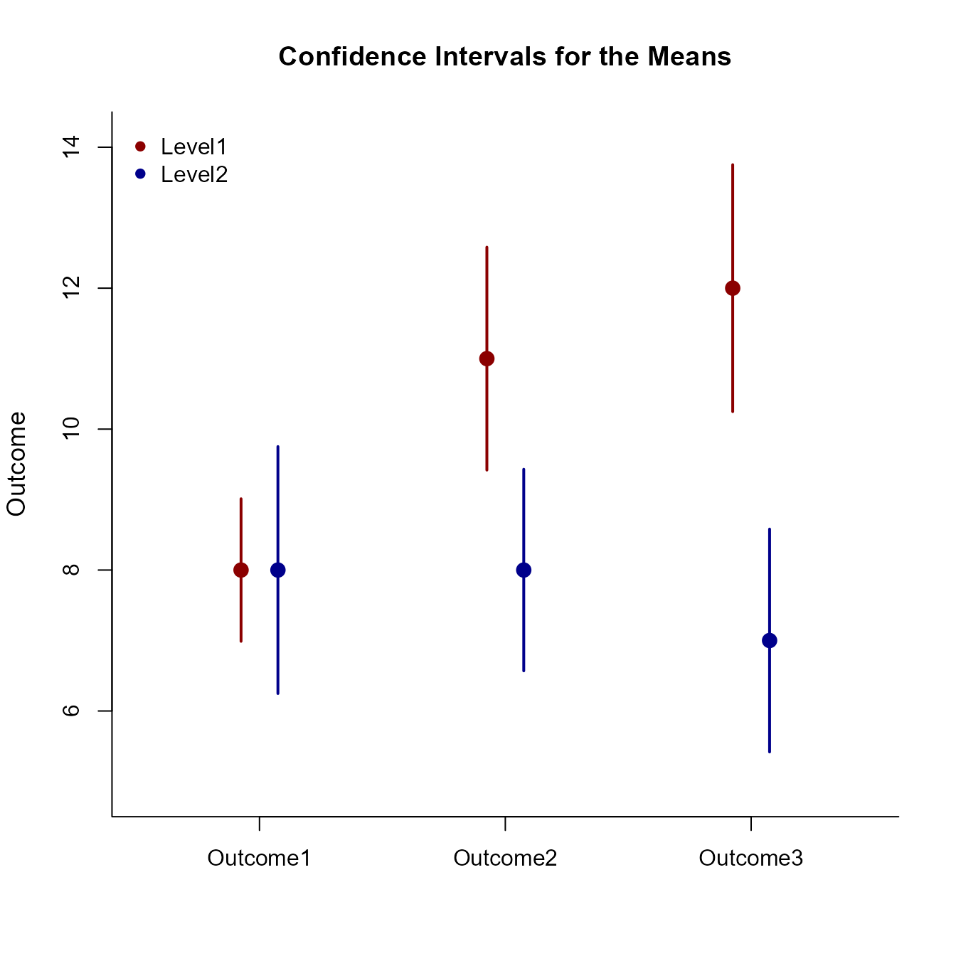
Plot the means and confidence intervals for the design as a whole.
(MixedMoments) |> plotFactorial(col = c("darkred", "darkblue"))
legend("topleft", inset = .01, box.lty = 0, pch = 16, legend = c("Level1", "Level2"), col = c("darkred", "darkblue"))
Analyses of the Omnibus Effects
The omnibus analysis usually consists of an Analysis of Variance.
Source Table
Get the source table associated with the main effects and the interaction.
(MixedMoments) |> describeFactorial(MixedCorr)$`Between Subjects`
Source Table for the Model
SS df MS
Blocks 106.667 1.000 106.667
Subjects 152.000 18.000 8.444
$`Within Subjects`
Source Table for the Model
SS df MS
Measures 30.000 2.000 15.000
Measures:Blocks 63.333 2.000 31.667
Residual 98.000 36.000 2.722Proportion of Variance Accounted For
Get estimates of the proportion of variance accounted for by each effect (along with their confidence intervals).
(MixedMoments) |> estimateFactorial(MixedCorr)$`Between Subjects`
Proportion of Variance Accounted For by the Model
Est LL UL
Blocks 0.412 0.114 0.595
$`Within Subjects`
Proportion of Variance Accounted For by the Model
Est LL UL
Measures 0.234 0.040 0.385
Measures:Blocks 0.393 0.163 0.528Significance Tests
Finally, test the various effects for statistical significance.
(MixedMoments) |> testFactorial(MixedCorr)$`Between Subjects`
Hypothesis Tests for the Model
F df1 df2 p
Blocks 12.632 1.000 18.000 0.002
$`Within Subjects`
Hypothesis Tests for the Model
F df1 df2 p
Measures 5.510 2.000 36.000 0.008
Measures:Blocks 11.633 2.000 36.000 0.000Analyses of the Simple Effects
As a follow-up to an Analysis of Variance, it is cusotmary to examine the simple effects (essentially a single-factor ANOVA separately across the levels of another factor).
Source Table
Get the source tables separately for the simple effects.
(MixedMoments) |> describeEffect(MixedCorr)$Level1
Source Table for the Model
SS df MS
Subjects 75.333 9.000 8.370
Measures 86.667 2.000 43.333
Error 40.667 18.000 2.259
$Level2
Source Table for the Model
SS df MS
Subjects 76.667 9.000 8.519
Measures 6.667 2.000 3.333
Error 57.333 18.000 3.185Proportion of Variance Accounted For
Get an estimate of the proportion of variance account for by the simple effect (and the confidence interval for that estimate).
(MixedMoments) |> estimateEffect(MixedCorr)$Level1
Proportion of Variance Accounted For by the Model
Est LL UL
Measures 0.681 0.389 0.772
$Level2
Proportion of Variance Accounted For by the Model
Est LL UL
Measures 0.104 0.000 0.282Significance Tests
Finally, test the simple effects for statistical significance.
(MixedMoments) |> testEffect(MixedCorr)$Level1
Hypothesis Test for the Model
F df1 df2 p
Measures 19.180 2.000 18.000 0.000
$Level2
Hypothesis Test for the Model
F df1 df2 p
Measures 1.047 2.000 18.000 0.372