Factorial Summary Traditional

This page examines a two-factor between-subjects (factorial) design using summary statistics input, focusing on omnibus and simple effects analyses.

Preliminary Tasks

Data Entry

This code inputs the group summaries and creates a single summary table

A1 <- c(N = 10, M = 8.000, SD = 1.414)
A2 <- c(N = 10, M = 11.000, SD = 2.211)
A3 <- c(N = 10, M = 12.000, SD = 2.449)
FactorialMomentsB1 <- construct(A1, A2, A3, class = "bsm")
A1 <- c(N = 10, M = 8.000, SD = 2.449)
A2 <- c(N = 10, M = 8.000, SD = 2.000)
A3 <- c(N = 10, M = 7.000, SD = 2.211)
FactorialMomentsB2 <- construct(A1, A2, A3, class = "bsm")
FactorialMoments <- combine(B1 = FactorialMomentsB1, B2 = FactorialMomentsB2)

Summary Statistics

This code confirms the descriptive statistics from the summary tables.

(FactorialMoments) |> describeMoments()

$B1

Summary Statistics for the Data

         N       M      SD
A1  10.000   8.000   1.414
A2  10.000  11.000   2.211
A3  10.000  12.000   2.449


$B2

Summary Statistics for the Data

         N       M      SD
A1  10.000   8.000   2.449
A2  10.000   8.000   2.000
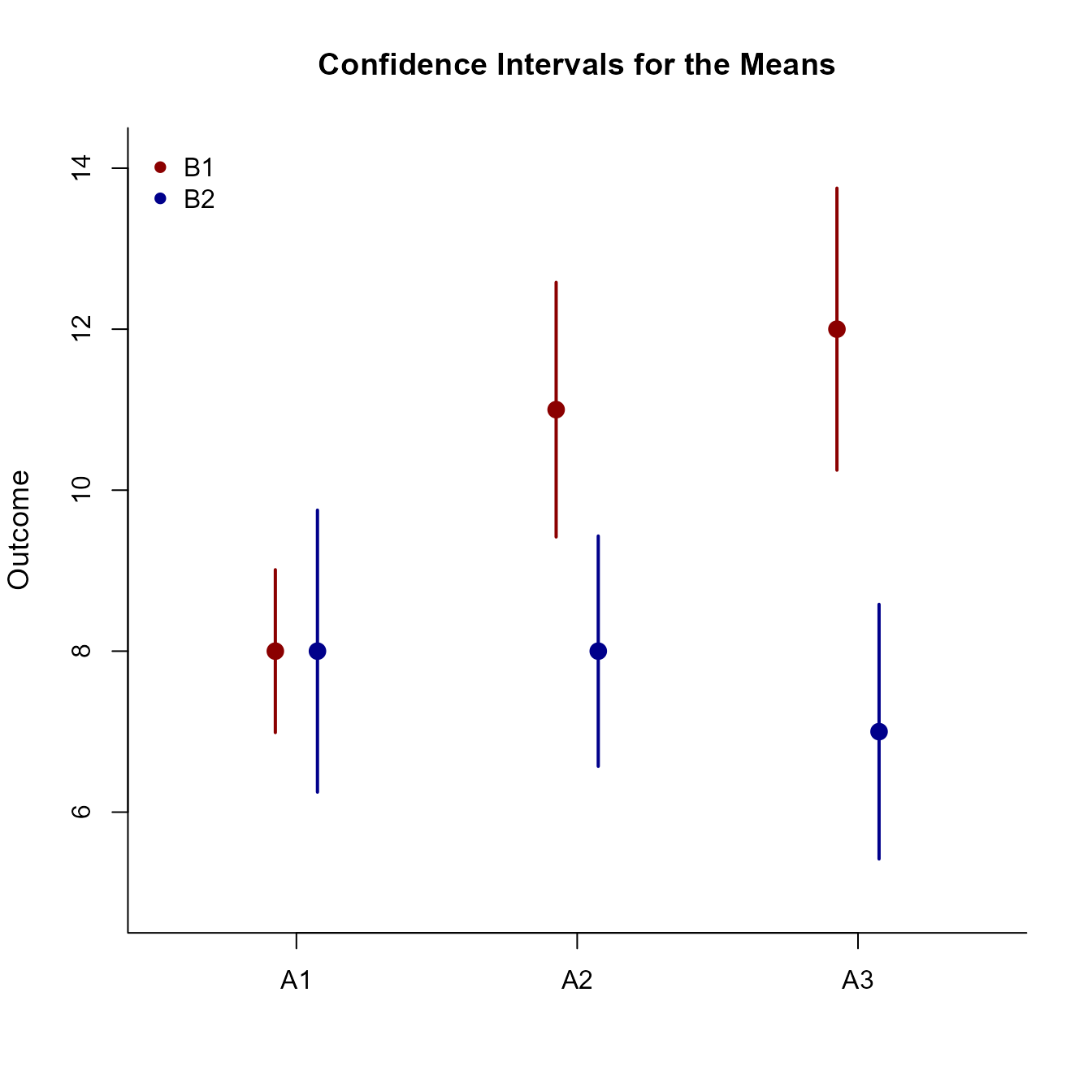
A3  10.000   7.000   2.211

Plot the means and their confidence intervals for the design as a whole.

(FactorialMoments) |> plotFactorial(col = c("darkred", "darkblue"))
legend("topleft", inset = .01, box.lty = 0, pch = 16, legend = c("B1", "B2"), col = c("darkred", "darkblue"))

Analyses of the Omnibus Effects

The omnibus analysis usually consists of an Analysis of Variance.

Source Table

Get the source table associated with the main effects and the interaction.

(FactorialMoments) |> describeFactorial()

Source Table for the Model

                   SS      df      MS
Factor        106.667   1.000 106.667
Blocks         30.000   2.000  15.000
Factor:Blocks  63.333   2.000  31.667
Residual      249.945  54.000   4.629

Proportion of Variance Accounted For

Get estimates of the proportion of variance accounted for by each effect (along with their confidence intervals).

(FactorialMoments) |> estimateFactorial()

Proportion of Variance Accounted For by the Model

                  Est      LL      UL
Factor          0.299   0.136   0.437
Blocks          0.107   0.000   0.176
Factor:Blocks   0.202   0.014   0.248

Significance Tests

Finally, test the various effects for statistical significance.

(FactorialMoments) |> testFactorial()

Hypothesis Tests for the Model

                    F     df1     df2       p
Factor         23.045   1.000  54.000   0.000
Blocks          3.241   2.000  54.000   0.047
Factor:Blocks   6.842   2.000  54.000   0.002

Analyses of the Simple Effects

As a follow-up to an Analysis of Variance, it is cusotmary to examine the simple effects (essentially a single-factor ANOVA separately across the levels of another factor).

Source Table

Get the source tables separately for the simple effects.

(FactorialMoments) |> describeEffect()

$B1

Source Table for the Model

             SS      df      MS
Between  86.667   2.000  43.333
Within  115.970  27.000   4.295


$B2

Source Table for the Model

             SS      df      MS
Between   6.667   2.000   3.333
Within  133.975  27.000   4.962

Proportion of Variance Accounted For

Get an estimate of the proportion of variance account for by the simple effect (and the confidence interval for that estimate).

(FactorialMoments) |> estimateEffect()

$B1

Proportion of Variance Accounted For by the Model

           Est      LL      UL
Factor   0.428   0.157   0.569


$B2

Proportion of Variance Accounted For by the Model

           Est      LL      UL
Factor   0.047   0.000   0.173

Significance Tests

Finally, test the simple effects for statistical significance.

(FactorialMoments) |> testEffect()

$B1

Hypothesis Test for the Model

             F     df1     df2       p
Factor  10.089   2.000  27.000   0.001


$B2

Hypothesis Test for the Model

             F     df1     df2       p
Factor   0.672   2.000  27.000   0.519